IPv4 Scan 2021 - Hop-Count Route Stability

October 16, 2021

masscan tracks the time to live of each packet coming from the host under scan.

⊕ Yes and no: they should not but some network devices will mangle the packets as they want, including setting arbitrary TTLs.

See the observations done in the TTL Boost post.

These time to live (TTL) are numbers between 0 and 255 set by the host. In its journey, the packet goes through different routers that each decrements by one the TTL.

Once a packet has a TTL of zero, the router will discard it.

⊕ Assuming that the packet goes straight-forward to us. If there are loops in the routing systems, the packet will loop between the devices going nowhere.
That’s the point of the TTL: to catch and drop packets looping around.

Of course the host set the TTL to some reasonable high number so the packet should reach to its destination (us) before reaching to zero.

We cannot know exactly which route/s the packets taken but we can count for how many hops they went through: any change in the hop-count and we will get different TTLs and that’s evidence that they taken different routes.

The inverse is not true: a constant hop-count does not imply that the route taken is the same, only the route/s have the same hops.

In this post I will continue exploring how much a route is stable in terms of hop-counts.

How much stable is a route in a burst?

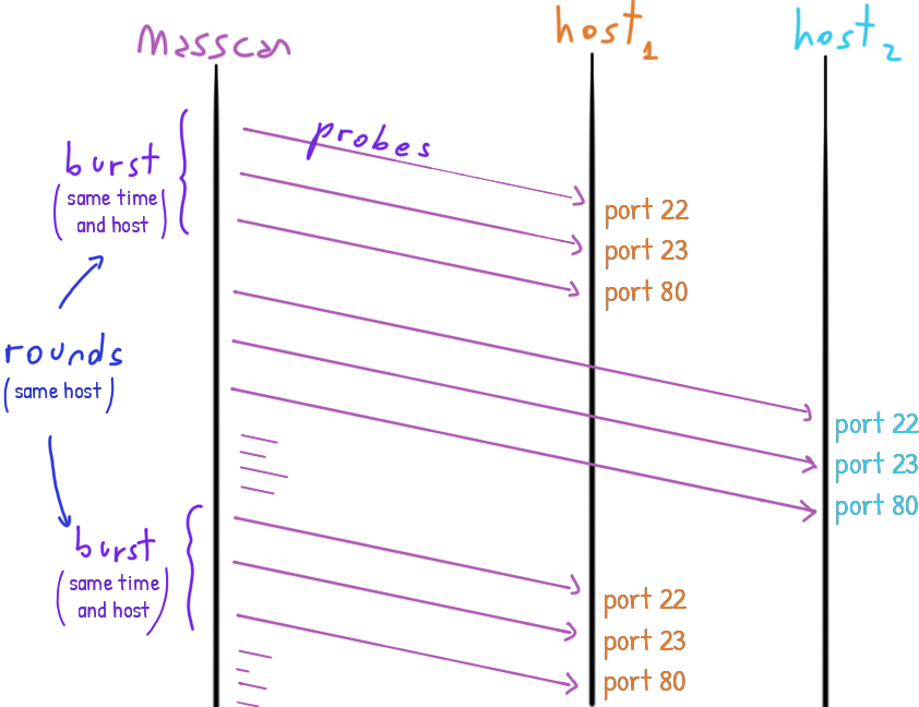
masscan scans the same host sending several probes at the same time in a burst.

As saw in a previous post, masscan may scan the same host more than once. We will call these rounds of bursts or just rounds.

TTLs extrema values for each short burst

Let’s review the short bursts first, the probes sent to a host at the same time:

julia> short_bursts_g = groupby(df, [:ip, :timestamp])
julia> short_bursts = combine(short_bursts_g, :ttl => minimum => :min, :ttl => maximum => :max)

Alternatively:

julia> short_bursts = combine(short_bursts_g, :ttl => (x -> [extrema(x)]) => [:min, :max])

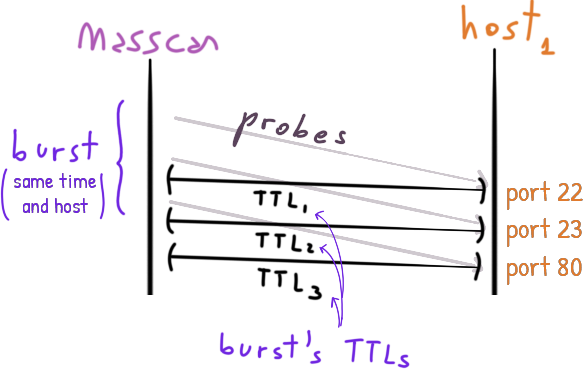⊕ For each response, the TTL is read and the minimum and maximum values are calculated for each burst.

This gives an idea of how different the TTL can be for probes sent in a short-elapsed burst.

The latter walks over the samples once calling the extrema function. However extrema is not compatible with DataFrames as is so we need to wrap it in an anonymous function (x -> [extrema(x)]).

This makes the latter much slower than the former, even if the former may walk over the samples twice.

Hop stability in short bursts

julia> countmap(short_bursts[:,:max] - short_bursts[:,:min])
Dict{Int32, Int64} with 6 entries:
  0 => 64801995
  1 => 68
  2 => 16
  3 => 1
  4 => 1
  7 => 4

The difference between the extremes, called the range, shows that the routes are quite stable, at least during the scan for a particular host.

The histogram shows that all the bursts have a TTL range of 0 except very few cases.

This means that the routes are stable but…

Keep in mind that the scans for a particular host in a particular time are like bursts: so it is reasonable that the routes didn’t change in such short period.

What would happen if we analyze now the stability for a longer period?

How much stable is a route in a longer period?

The dataset has scans to the same host at different time, what we call rounds.

We can do a second groupby + combine taking the minimum of the minimum TTLs and the maximum of the maximum TTLs to have the range per host, regardless of the timestamp, hence capturing some statistics for each round.

However we need to filter out the groups of scans to the same host that have only one timestamps: we want to compare rounds at different time and having a single round defeats the purpose.

These are scans to a host that were done in a single burst and we don’t have different burst at different time to compare with!

⊕ julia> hist_biased[0] - hist_unbiased[0] 29349509

To give you an idea of how much the bias towards stable routes is (aka range of 0).

If we left those, our analysis will be biased toward stable routes (range of 0).

Rounds of bursts

julia> all_rounds_g = groupby(short_bursts, :ip)

julia> rounds_g = filter(sdf -> nrow(sdf) != 1, all_rounds_g)
julia> rounds_ttl = combine(rounds_g, :min => minimum => :min, :max => maximum => :max)

julia> hist_unbiased = countmap(rounds_ttl[:,:max] - rounds_ttl[:,:min])
Dict{Int32, Int64} with 217 entries:
  56  => 50
  35  => 221
  60  => 597
  220 => 4
  67  => 5813
  73  => 75
  115 => 3
  112 => 4
  185 => 85
  ⋮   => ⋮

⊕ Yes, the (-) is the binary operator minus or subtraction that is applied row by row to the maximum and minimum values (:max and :min columns).

Hop stability in longer periods

Okay, the situation is quite different!

julia> multirounds_range = select(rounds_ttl, :ip, [:max, :min] => (-) => :range)

julia> describe(multirounds_range, :mean, :std, :min, :q25, :median, :q75, :max, cols=:range)
1×8 DataFrame
 Row │ variable  mean      std      min    q25      median   q75     max
─────┼──────────────────────────────────────────────────────────────────────
   1 │ range     0.634406  6.73528      0      0.0      0.0      0.0   239

So 75% of the samples have a range of 0. Let’s analyze the dataset without them:

julia> not_perfectly_stable = filter(:range => !=(0), multirounds_range)

julia> quite_stable = filter(:range => <=(7), not_perfectly_stable)
julia> describe(quite_stable, :mean, :std, :min, :q25, :median, :q75, :max, cols=:range)
 Row │ variable  mean     std      min    q25      median   q75      max
─────┼─────────────────────────────────────────────────────────────────────
   1 │ range     1.77117  1.39118      1      1.0      1.0      2.0    7


julia> unstable = filter(:range => >(7), not_perfectly_stable)
julia> describe(unstable, :mean, :std, :min, :q25, :median, :q75, :max, cols=:range)
 Row │ variable  mean     std      min    q25      median   q75      max
─────┼─────────────────────────────────────────────────────────────────────
   1 │ range     85.5505  62.5483      8     62.0     64.0    127.0   239

So it seems that the difference between TTLs for the same host is quite concentrated on 0 and closer, up to 7, as the mean 1.77117 and the standard deviation 1.39118 shows.

From there the differences are spread over the 8 to 239 range. The mean is around the middle of the range and the standard deviation is approx one quarter so the values are really spread.

⊕ In the dataset we have a slightly more unique hosts: 43056596. The difference is due the filtering that we did above but it does not change the results.

There are only 172217 samples of 43056567 unique hosts so the unstable represents only 0.39998%.

Bursts over longer periods but for how long?

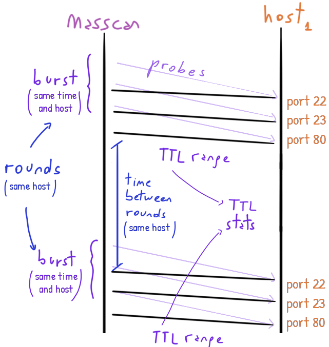⊕ For each burst we calculate its TTL range.

From there, a bunch of statistics can be calculated about the TTL ranges for the same hosts giving us an idea of the stability of the route to it.

Can we conclude that the routes are 99% of the time stable?

Well, yes but we are making an assumption: when we have two or more bursts to the same host we are assuming that those happen at different moments but… what do we mean by different moments?

Certainly, a difference of a few seconds does not change anything by real.

What we want is to measure the changes in the TTLs between bursts that happen at hours of difference.

So, let’s check how spread are the timestamps of the grouped by :ip, aka how spread are the bursts:

julia> rounds_spread = combine(rounds_g, :timestamp => std)
julia> describe(rounds_spread, :mean, :std, :min, :q25, :median, :q75, :max, cols=:timestamp_std)
 Row │ variable       mean     std      min       q25      median   q75      max
─────┼─────────────────────────────────────────────────────────────────────────────────
   1 │ timestamp_std  51768.5  32284.3  0.707107  25612.8  49328.5  73464.1  1.52706e5

So we have bursts that happen one after the other, roughly with 0.707 seconds of difference.

But most of the burst happen with several minutes, even hours of difference.

The 25-quantile, that represents the value of the first quarter of the samples, is of 25612.8 seconds, a little more than 7 hours.

Conclusions

So with these so-spread bursts and the so-little changed difference in the TTLs we can conclude that most of the hop-count routes are stable.

We cannot say anything about the real routes that the packets took but we can know that the count of hops that they passed through remained constant.

Related tags: pandas, julia, statistics, seaborn